Moment-guided edge sampling
Connecting local edge edits to global graph structure through spectral moments.
This post shares deeper reflections that are not suitable for a research paper. It also provides foundational knowledge to make the paper easier to understand.
This post covers:
- Intention: Why I set out to do this.
- Foundational knowledge:
- What are closed walks and moments?
- What do they have to do with Steel Ball Run: JoJo’s Bizarre Adventure?
- Proposed method: A deeper explanation of the combinatorial and low-rank approaches.
- Results: A brief discussion of the results.
This is not a summary of the paper. You can read it alongside the paper to better understand the work.
0. Intention
Many graph learning studies do not explicitly mention sampling, but they employ it by default. In graph contrastive learning, for example, we can create two views by randomly dropping edges or editing edges to widen the spectral gap. These choices may improve performance, but which perturbation is optimal, and why?
As a rough analogy, I view the graph itself as an initialized deep learning model. Changing its structure to create better contrastive views is like tuning a model’s parameters.
From this perspective, many proposed GCL (graph contrastive learning) methods resemble adjusting model weights by hand in search of a global optimum. Even gradient descent cannot guarantee one. Yet a small improvement may lead to a paper, although it could be just one of millions of local optima. Contrastive learning is only one example; the same perspective applies to other graph tasks that use sampling.
This leads to the question behind this project: What is the optimal perturbation for graph learning? Finding a well-justified optimum and explaining why it works are difficult. Could we start with a less ambitious goal? My first step is to develop somthing like gradient descent on graphs. Each update would add or delete edges instead of changing model parameters.
If we can find (1) a measure that represents graphs much like model parameters, and (2) a sampling method that controls the direction and size of each step in that space, we could map the performance landscape and search for an optimum. This project grew from that idea. We use moments to measure graphs and propose moment-guided sampling to guide this graph “gradient descent” through moment space.
1. Closed walks and moments
Closed walks and moments can be the way to represent graphs, so let us first understand intuitively.
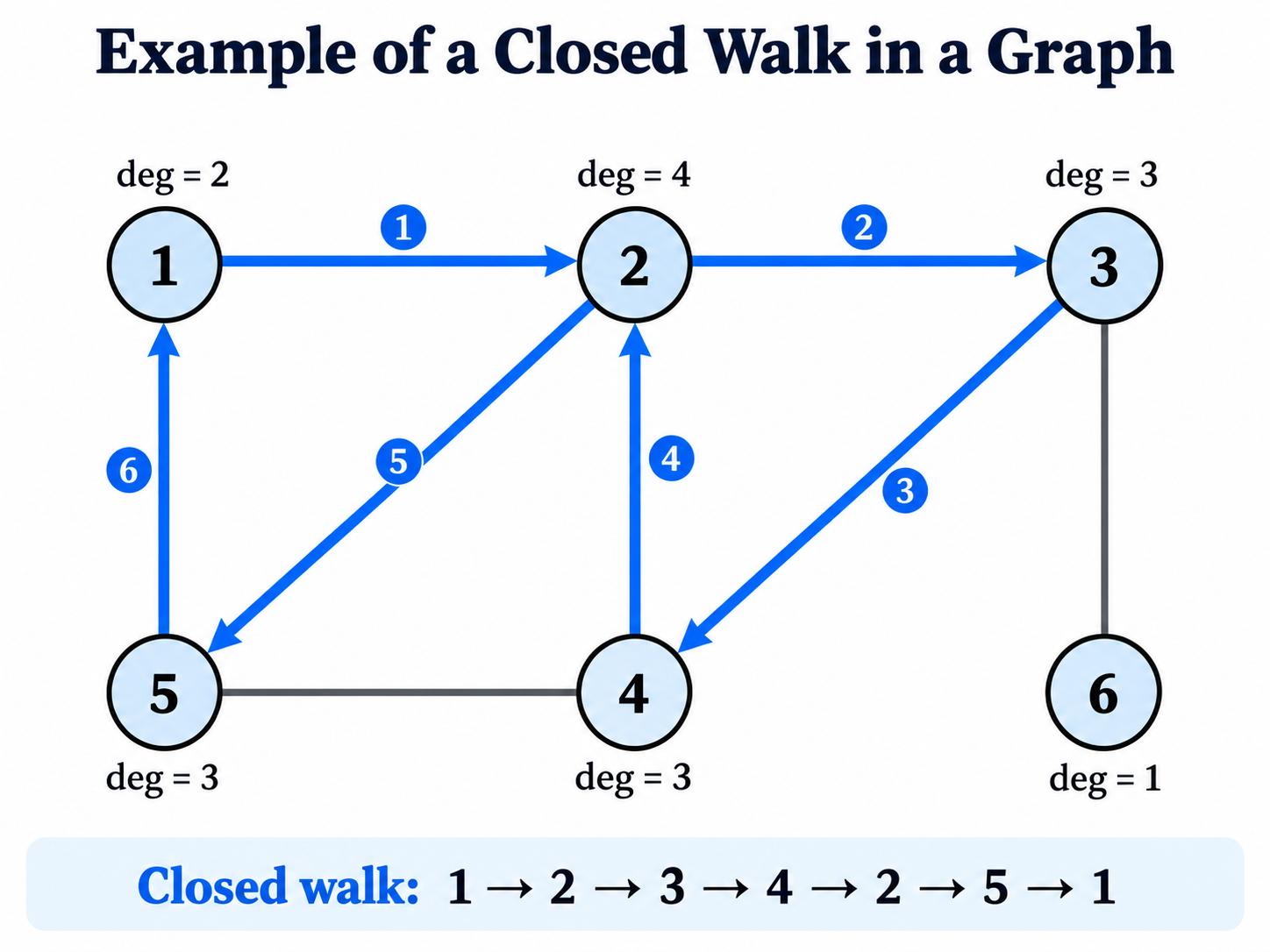
A closed walk starts and ends at the same node.
- It can pass through the same node or edge more than once.
- Its length is the number of steps along edges, counting repeated steps.
- We can regard it as a loop or a spining ball; imagine a spining ball moving along the edges and returning to where it started.
In the figure below, 1 → 2 → 3 → 4 → 2 → 5 → 1 is a closed walk of length 6. The shorter route 1 → 2 → 5 → 1 is a closed walk of length 3.
A graph without isolated nodes can be represented by a finite collection of closed walks that covers every case. And combining these walks recovers the original graph. This gives us a way to describe a graph through its closed walks.
Directly describing discrete walk set is difficult, therefore we turn to moments, because Moments summarize closed walks:
- Without degree weighting: The $k$-th moment, $m_k = \frac{1}{n}\mathrm{Tr}(A^k)$, is the average number of length-$k$ closed walks starting at a node. Here, $A$ is the adjacency matrix and $n$ is the number of nodes.
- With degree weighting: The $k$-th moment, $m_k = \frac{1}{n}\mathrm{Tr}(P^k)$, is the average probability of returning to the starting node after $k$ steps. Here, $P = AD^{-1}$ is the random-walk transition matrix, and $D$ contains the node degrees on its diagonal. Equivalently, this moment is a normalized sum of weighted length-$k$ closed walks.
Therefore, moments serve as statistics of closed walks, which can describe graphs with multiple orders. Using several moments, such as $(m_2, m_3, m_4)$, gives us a compact description of a graph, though it does not uniquely determine its structure. The example below is from Jin and Zafarani (2020)
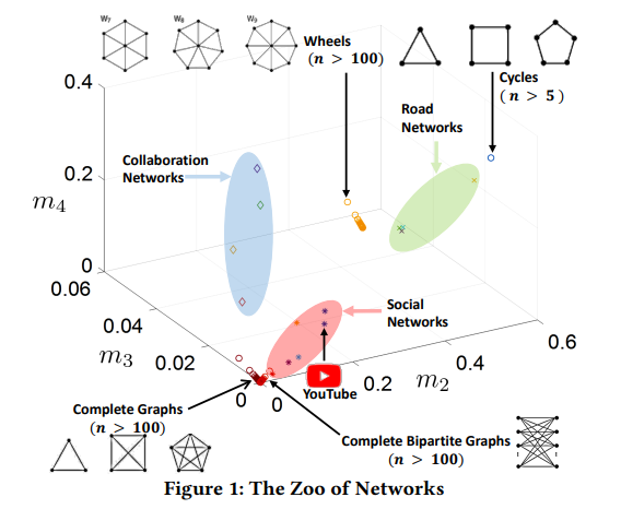
Can we design a sampling method that adds or deletes edges to move a graph in a chosen direction through this space? For example, by reducing the $m_2$ and $m_4$ of road networks to make them more similar to social networks. How would we design such a method? And how can we measure the “gradient” of each edge addition or deletion?
2. The gradient $\Delta m_k(e)$
The “gradient” of an edge edit (e.g., edge addition and edge deletion) describes the direction and size of the change it causes in a graph’s moments. Knowing these changes helps us choose edge additions or deletions that move the graph toward a target in moment space. We use $\Delta m_k(e)$ to denote the change in the $k$-th moment after deleting edge $e$.
Let us first build an intuition for $\Delta m_k(e)$. The next two sections explain how to compute it.
The panel below shows seven classic graphs, each in a different color. For every edge, we compute $\Delta m_2(e)$ and $\Delta m_3(e)$, then plot the density of their “gradient” directions. We also place eight local motifs at their corresponding directions. In each motif, the red edge marks the edge being deleted.
Take the cycle graph as an example. All edges have the same structural role, and deleting any edge gives $\Delta m_2(e) > 0$ and $\Delta m_3(e) = 0$. All edges therefore point in the $0^\circ$ direction.
This example shows that $\Delta m_k(e)$ can help us both control graph structure and interpret individual edges through their local motifs.
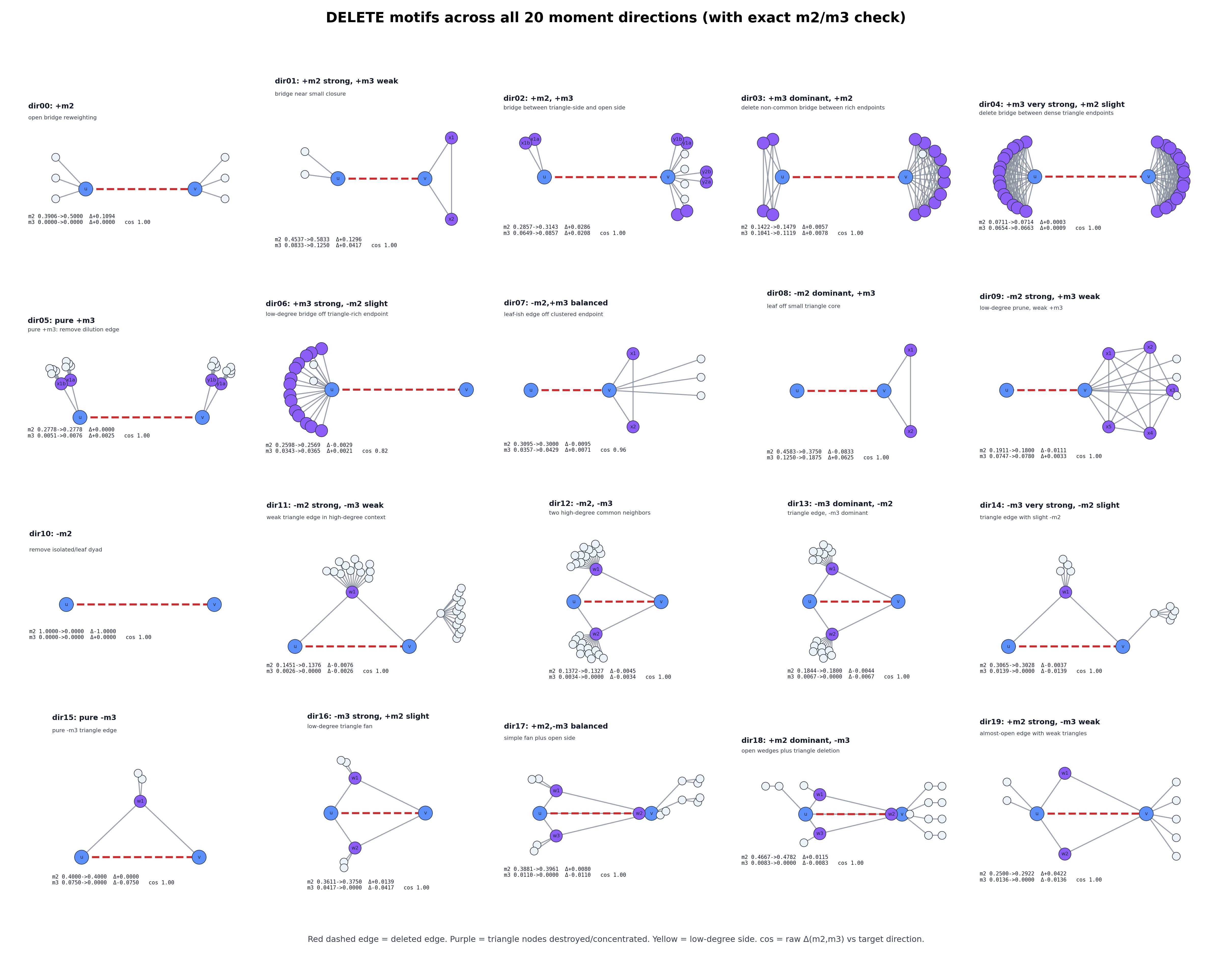
We provide more examples below. We divide the full $360^\circ$ into 20 angular bins and show one example motif in each bin for both edge addition and deletion. In these examples, corresponding additions and deletions produce approximately opposite directions in moment space. For example, compare dir00 for deletion with dir10 for addition, or dir09 for deletion with dir19 for addition.
Below are the local motifs for edge deletion. Click the image to open the PDF.
Below are the local motifs for edge addition. Click the image to open the PDF.
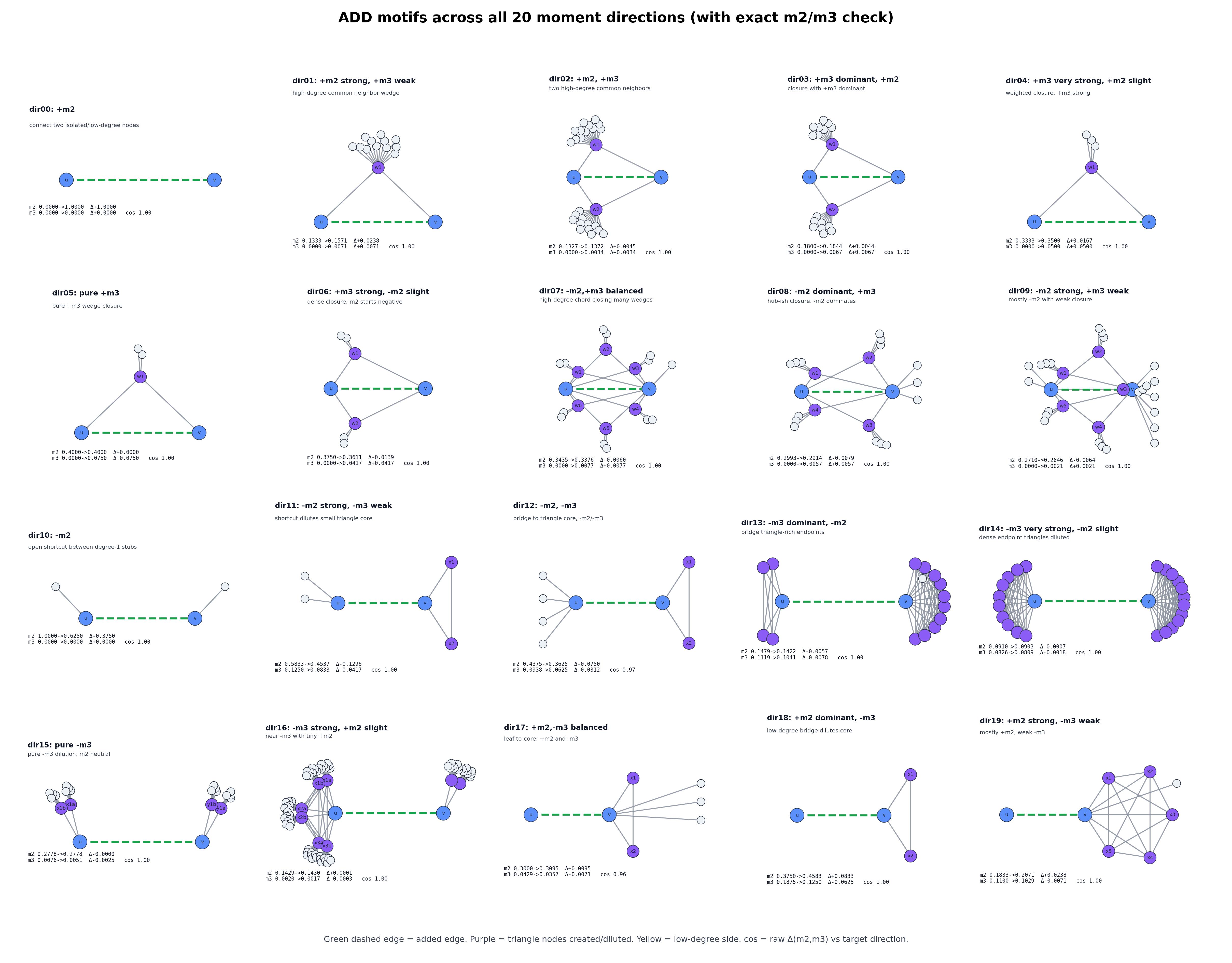
Now that we have an intuition for the “gradient” $\Delta m_k(e)$, let us discuss the main idea behind computing it.
2.1 Enumerating all affected cases: combinatorial method
Since moments summarize closed walks, we can compute $\Delta m_k(e)$ by identifying the affected walks and adding up their contributions to the change.
The second and third moments are:
\[m_2 = \frac{1}{n}\mathrm{Tr}(P^2) = \frac{2}{n} \sum_{\{i, j\}\in E} \frac{1}{d_i d_j} \tag{1} \label{eq:m2}\] \[m_3 = \frac{1}{n}\mathrm{Tr}(P^3) = \frac{6}{n} \sum_{\{i, j, k\}\in \triangle} \frac{1}{d_i d_j d_k} \tag{2} \label{eq:m3}\]Here, $n$ is the number of nodes, $d_i$ is the degree of node $i$, and each triangle is counted once in $\triangle$.
In the example below, the red edge $e$ connects A and B. Let us follow the combinatorial approach to compute $\Delta m_2(e)$ and $\Delta m_3(e)$ after deleting it.
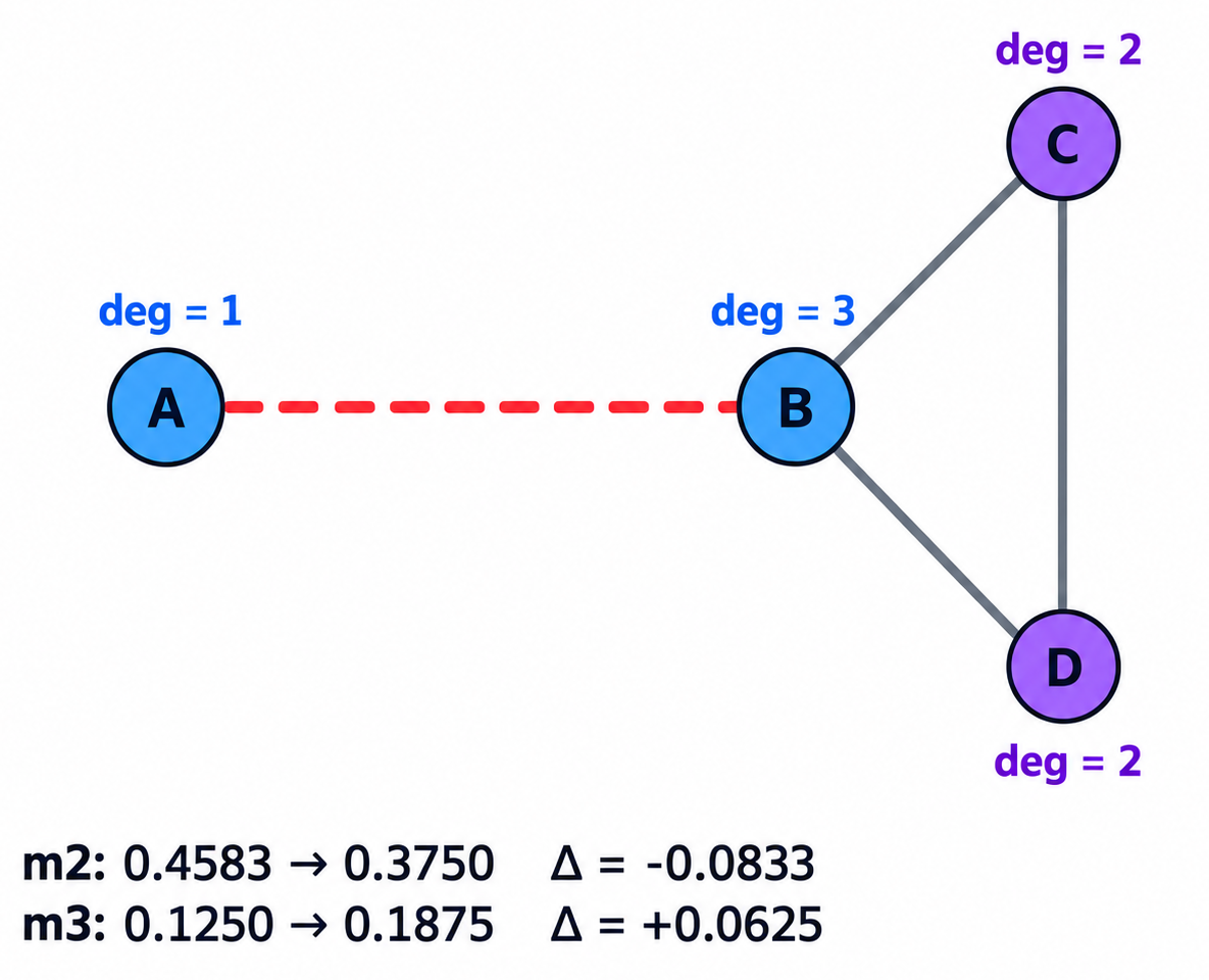
Deleting A–B leaves A isolated and reduces B’s degree from 3 to 2. We keep A in the graph, so $n$ remains unchanged.
For $m_2$, two changes occur:
- Some closed walks disappear. The walks A → B → A and B → A → B are removed, eliminating the A–B term from Equation $\eqref{eq:m2}$.
- Other closed walks are reweighted. Since B’s degree decreases, the weights of the walks along B–C and B–D increase.
Adding these changes gives $\Delta m_2(e)$.
For $m_3$, we consider the same two effects:
- Some closed walks may disappear. This happens when the deleted edge belongs to a triangle. In this example, A–B belongs to no triangle, so no length-3 closed walks are removed.
- Other closed walks are reweighted. The triangle B–C–D remains, but its contribution to Equation $\eqref{eq:m3}$ increases because B’s degree decreases.
Adding these changes gives $\Delta m_3(e)$. The same idea also applies to edge addition.
For low-order moments, this approach makes $\Delta m_2(e)$ and $\Delta m_3(e)$ easy and efficient to compute. But what about higher-order moments, such as $m_4$ and $m_5$? Longer closed walks involve more complex patterns, making it harder to enumerate every case.
Can we instead derive a general formula that computes $\Delta m_k(e)$ efficiently without enumerating these cases?
2.2 The spin of closed walks: low-rank method
In Steel Ball Run: JoJo’s Bizarre Adventure, the Zeppeli family masters the rotation of steel balls. This idea of rotation also offers an intuitive way to understand how we compute $\Delta m_k(e)$.

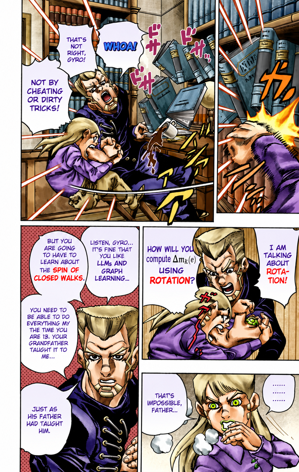
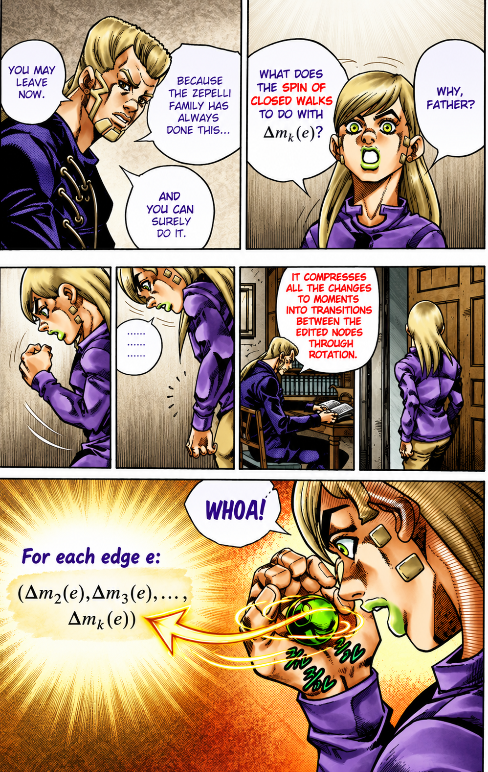
Let us use an example to connect this intuition to the formulas in the paper.
As discussed earlier, moments summarize closed walks. After deleting edges $e_1, \ldots, e_m$, $\Delta m_k(e_1, \ldots, e_m)$ captures changes in walks that visit at least one edited endpoint. By rotating a closed walk, we can choose an edited endpoint as its starting and ending node. We can then split the walk into segments connecting edited endpoints.
Suppose we delete $e_1 = (1,2)$ and $e_2 = (4,5)$ and want to compute $\Delta m_5(e_1, e_2)$. The edited endpoints are ${1,2,4,5}$.
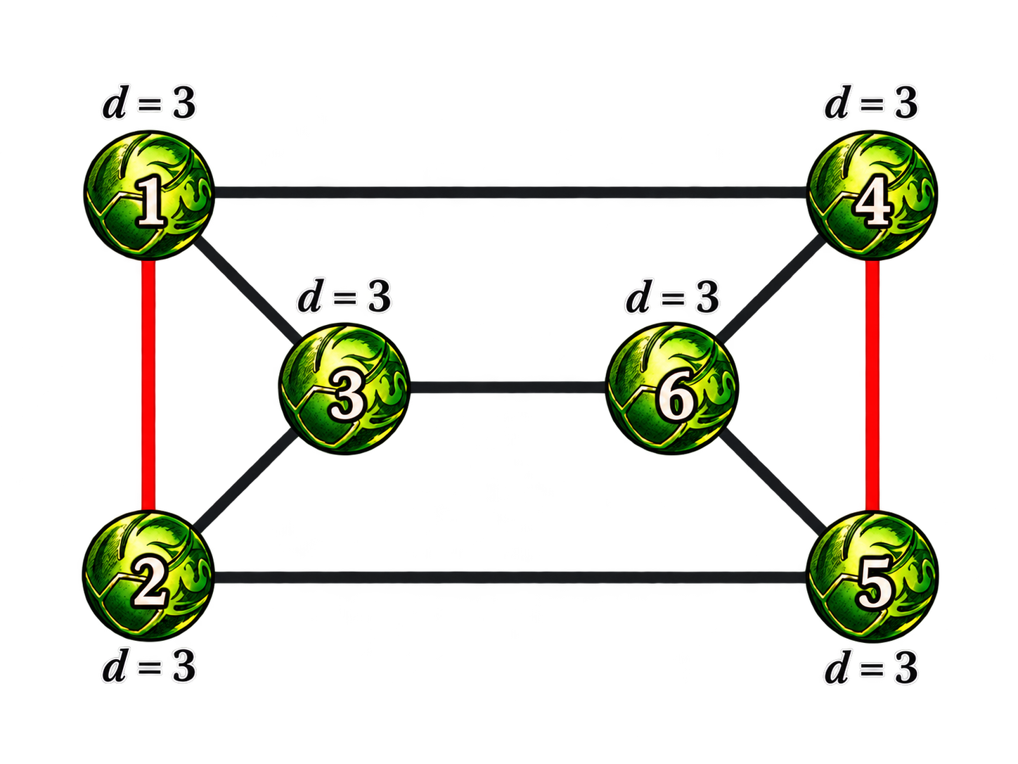
One affected closed walk is 3 → 1 → 4 → 5 → 6 → 3. Rotating it gives 1 → 4 → 5 → 6 → 3 → 1, which starts and ends at an edited endpoint. We can split it into three segments:
- 1 → 4: one step.
- 4 → 5: one step.
- 5 → 1: three steps from 5 back to 1.
This gives us an endpoint pattern: 1 → 4 → 5 → 1, with segment lengths 1, 1, and 3.
The benefit is that we can group individual walks into more general patterns. Instead of listing every intermediate route, we specify the edited endpoints at the segment boundaries and the length of each segment. Entries of powers of $P$ then sum the weighted walks connecting those endpoints.
For example, both 1 → 4 → 5 → 6 → 3 → 1 and 1 → 4 → 5 → 2 → 3 → 1 fit this pattern. They share the first two segments but take different three-step routes from 5 back to 1.
Rotation therefore lets us express affected closed walks through edited endpoints. We can then aggregate their contributions through endpoint-to-endpoint transitions, rather than enumerate every walk.
3. Results
Please see the paper for the full results. Here, I highlight three findings:
- Interpretable structural signatures: Moment changes help explain individual edges and provide graph fingerprints.
- Connections to graph properties: Moments relate to properties such as clustering coefficients and degree structure.
- Graph learning: Moment-guided sampling enables analysis and improvement of graph learning.
This project is a first step toward my original intention. We represent graphs in moment space and develop a sampling method that acts as a “gradient calculator”.
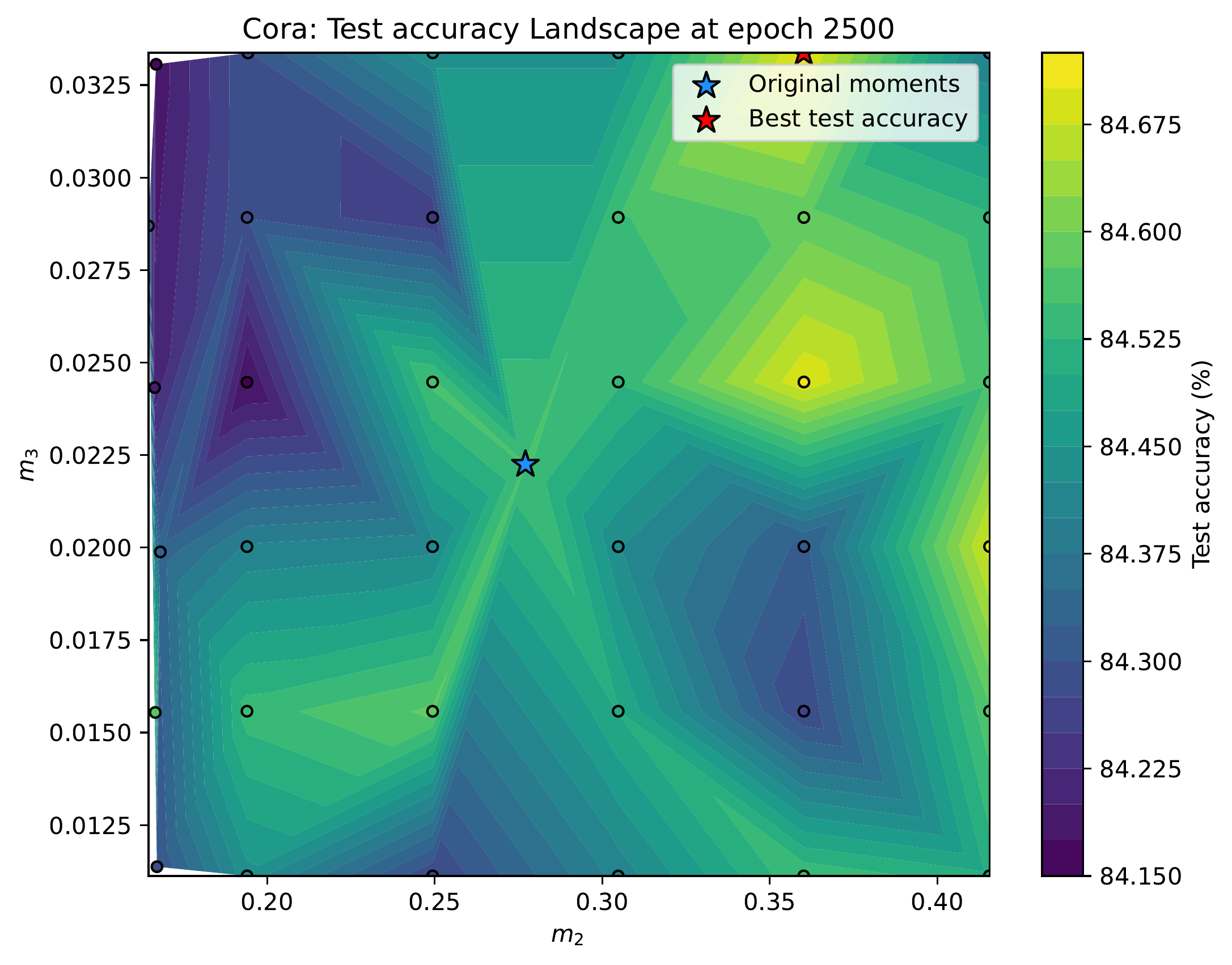
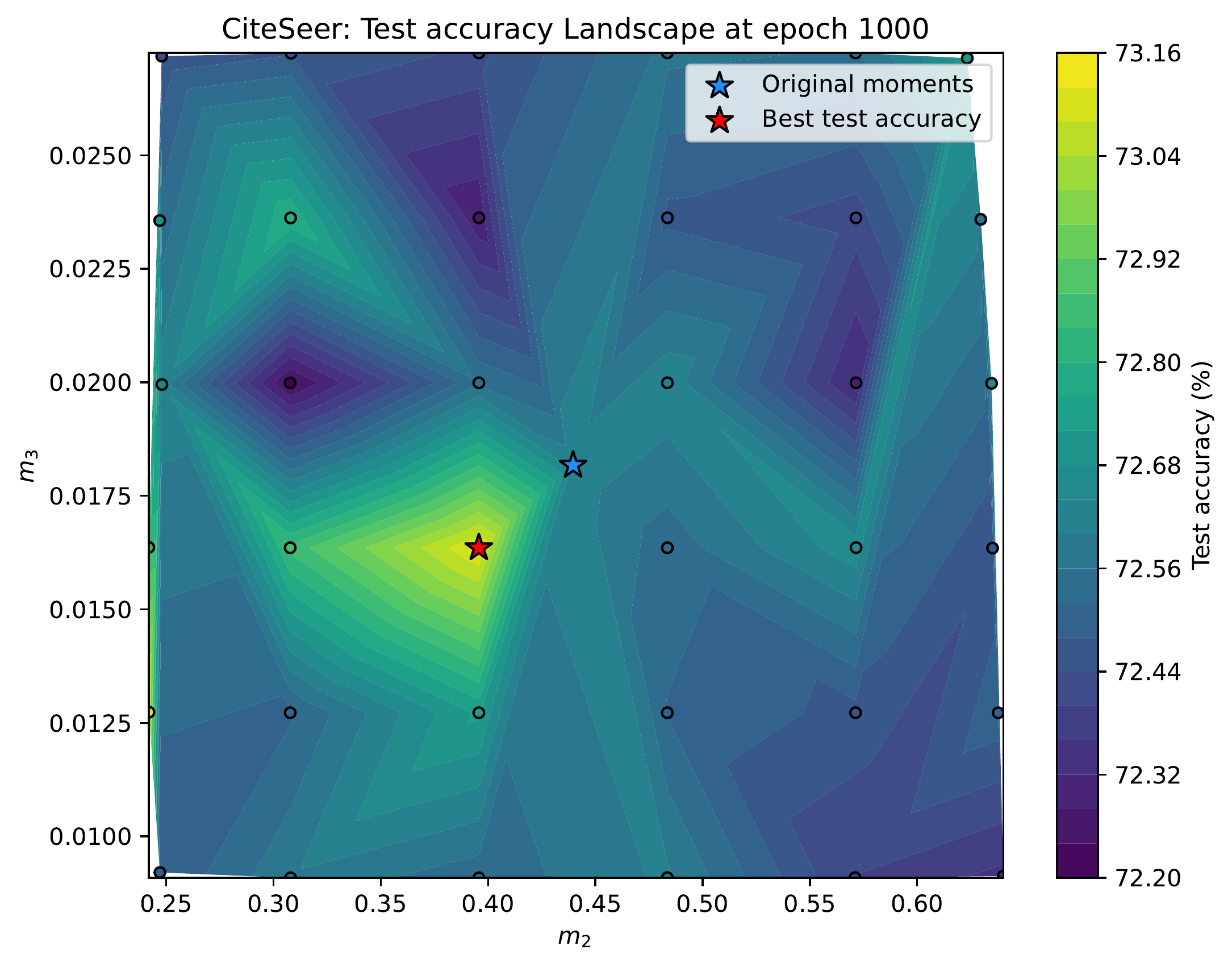
The appendix explores how performance varies across moment space. We use moment-guided sampling to move graphs toward different moment targets, use the resulting graphs as augmented views in graph contrastive learning, and evaluate them on an unsupervised node classification task.
The test accuracy landscapes show that the best observed performance occurs away from the original moments, although preserving the original moments remains competitive.
BibTeX
-
@article{cai2026moment,
  title = {Moment-guided edge sampling},
  author = {Cai, Weibin and Zafarani, Reza},
  journal = {arXiv preprint arXiv:2609.30472},
  year = {2026},
}
Enjoy Reading This Article?
Here are some more articles you might like to read next: